Simple Forecasting
Timeseries financial forecasting
Recently , I have been looking into various ways to forecast a time series dataset. This is an old pursuit in the field of statistics and there are many well known ways to achieve this.
In this post I will demonstrate a very basic (Naive) approach of forecasting a quarterly dataset of sales figure, by using previous 4 years (16 quarters) and forecasting/predicting the next 1 year of sales aggregate.
I am going to use pandas for basic utilities and sklearn for simple linear-regression model.
Prepare data
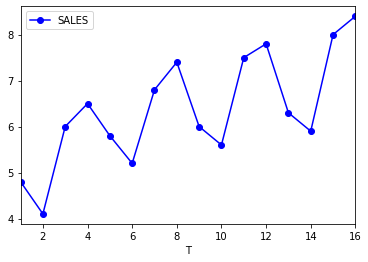
I have created data frame directly in the code like shown below.
df = pd.DataFrame(
    {
        'T': pd.RangeIndex(1, 17).to_series(),
        'YEAR': [1,1,1,1,2,2,2,2,3,3,3,3,4,4,4,4],
        'QUARTER': [1,2,3,4,1,2,3,4,1,2,3,4,1,2,3,4],
        'SALES': [4.8,4.1,6.0,6.5,5.8,5.2,6.8,7.4,6.0,5.6,7.5,7.8,6.3,5.9,8.0,8.4],
    }
)
Moving and Centred average
Moving averages is a technique used to smoothen the data out , this is a very simple way to do seasonal adjustment. In pandas, we will use rolling function with the window size of 4. The seasonal cycle in this case is known to last 4 quarters.
df["MA"] = df.SALES.rolling(window=4).mean().shift(-1)
Since our window size (4)is even, we will need to centre the data as well.
df["CA"] = df.MA.rolling(window=2).mean().shift(-1)
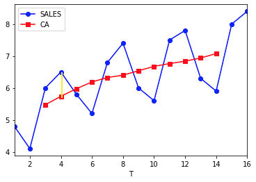
Seasonal and Irregular Components (StIt)
We are going to extract Seasonal and Irregular components by simply dividing the sales value with the Centred Average.
df["StIt"] = df.SALES/df.CA
Here is a helpful method to populate description for Seasonal and irregular figures, (optional)
def StItDescription(v):
    if pd.isnull(v):
        return v

    direction = "above"
    if v < 1:
         direction = "below"

    v = round(abs((1 - v) * 100))
    return "{v}% {d} baseline.".format(v=v,d=direction)
df["StItD"] = df["StIt"].apply(lambda x:StItDescription(x))
So take a moment to understand what these values really indicate. The number 1.095890 indicate that in year 1, quarter 4 the seasonal and irregular components were 13% above (yellow line in figure below) the smoothened baseline, or year 3 quarter 3 the seasonal and irregular components were 11%(rounded) above baseline.
Seasonal components
Before we start removing the seasonal and irregular components we need to smoothen these values by taking the average of StIt column across each quarter, this will give us just the seasonal component S(t).
averages = df.groupby("QUARTER",as_index=True)["StIt"].mean()
QUARTER
1    0.932200
2    0.837759
3    1.093349
4    1.143305
df = df.join(averages.rename("St"),on="QUARTER")
DeSeasonalize
Next, we use the yearly averages (St) and divide Yt (sales) to get deseasonalise values. This column has no seasonality or irregularity components now.
df["DeSeasonalize"] = df.SALES/df.St
Linear regression and Trend Prediction (Tt)
Next we use , good old, linear regression to do some actual trend prediction for trend values, note how the independent variable (X) is simply a count (1,2,3…….16) and the dependent variable (Y) is the deseasonalised variable.
linear_regressor = LinearRegression()
Y = df["DeSeasonalize"].values.reshape(-1, 1)
X = df["T"].values.reshape(-1, 1)
linear_regressor.fit(X, Y)
[linear_regressor.coef_,linear_regressor.intercept_]
The coffecients returned in this case are
coef_ = 0.14713872
intercept_ = 5.09961009
df["Trend(Tt)"] = linear_regressor.predict(X)
Forecasting
We are using a classical multiplicative model to forecast, which basically says :
Forecasted value as a given time Y(t) is a product of seasonal component S(t) times irregular component I(t) times trend component (Tt). $$ Y_t = S_t I_tT_t $$ Let’s test the formula against the actuals by forecasting for past values, note we will prefer the smoothened version of the Seasonal and Trend component in the formula df[“st”], instead of df[“StIt”]
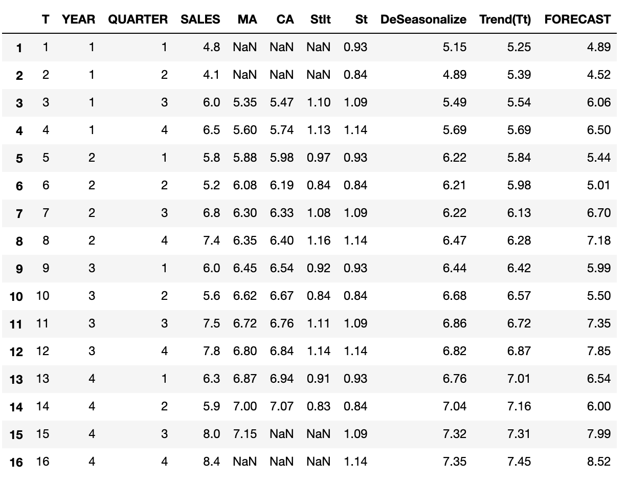
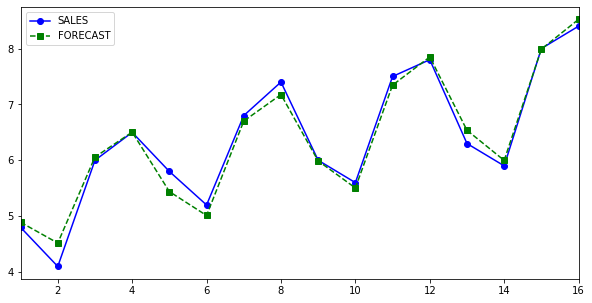
df["FORECAST"] = df["St"] * df["Trend(Tt)"]
with pd.option_context('precision', 2):
    display(df.head(16))
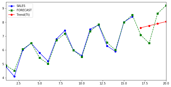
Here is a view of what has been achieved so far, Sales column is actuals and Forecast is predicted.
Forecasting Future
Now that all the hard work has been done, predicting future is relatively straightforward. We are going to aim for next 1 year i.e. next 4 quarters as going any further won’t be appropriate.
#Create next 4 quarters for year 5.
future = pd.DataFrame(
    {
        'T': pd.RangeIndex(17, 21).to_series(),
        'YEAR': [5,5,5,5],
        'QUARTER': [1,2,3,4],
    }
)
#Fill int the seasonality values.
future = future.join(averages.rename("St"),on="QUARTER")
X = future["T"].values.reshape(-1, 1)
#Predict Trend from DeSeasonalized components.
future["Trend(Tt)"] = linear_regressor.predict(X)
#Forecast the next 4 quarters based on seasonality and trend.
future["FORECAST"] = future["St"] * future["Trend(Tt)"]

#select only the relevant columns.
training = df[["T","CA","SALES","FORECAST","YEAR","QUARTER"]]
#extend dataframe to contain all 5 years.
merged = pd.concat([training,future], axis=0,copy=True,sort=True)
Here is the final plot.